Greenwicher's WikiFRM - Quantitative Analysis 2017-08-29

[Last Update: Oct 27, 2017]

The Time Value of Money

Time Value of Money Concepts and Applications

• compound interest or interest on interest
• future value
• present value

Using a Financial Calculator

• learn to solve the TVM (time value of money) problems

Time Lines

• discounting/compounding
• cash flows occur at the end of the period depicted on the time line
• required rate of return / discount rate / opportunity cost
• noimal risk-free rate = real risk-free rate + expected inflation rate
• required interest rate on a security = noimal risk-free rate + default risk premium + liquidity premium + maturity risk premium

Present Value of a Single Sum

Annuities

• ordinary annuity

Present Value of a Perpetuity

PV and FV of Uneven Cash Flow Series

Solving TVM Problems When Compounding Periods are Other Than Annual

Probabilities

Random Variables

LO 15.1: Describe and distinguish between continuous and discrete random variables.

Distribution Functions

LO 15.2: Define and distinguish between the probability density function, the cumulative distribution function, and the inverse cumulative distribution function.

Discrete Probability Function

LO 15.3: Calculate the probability of an event given a discrete probability function.

Conditional Probabilities

LO 15.6: Define and calculate a conditional probability, and distinguish between conditional and unconditional probabilities.

Independent and Mutually Exclusive Events

LO 15.4: Distinguish between independent and mutually exclusive events.

Calculating a Joint Probability of Any Number of Independent Events

LO 15.5: Define joint probability, describe a probability matrix, and calculate joint probabilities using probability matrices.

Probability Matrix

Basic Statistics

Measure of Central Tendency

LO 16.1: Interpret and apply the mean, standard deviation, and variance of a random variable.

LO 16.2: Calculate the mean, standard deviation, and variance of a discrete random variable.

• population mean / sample mean

Expectations

LO 16.3: Interpret and calculate the expected value of a discrete random variables.

LO 16.4: Calculate the mean and variance of sums of variables.

Variance and Standard Deviation

Covariance and Correlation

LO 16.5: Calculate and interpret the covariance and correlation between two random variables.

correlation measures the strength of the linear relationship between two random variables

Interpreting a Scatter Plot

Moments and Central Moments

• skewness (standardized third central moment): evaluate whether the distribution is symmetric
• kurtosis (standardized fourth central moment): refers to the degree of peakedness or clustering in the data distribution

LO 16.6: Describe the four central moments of a statistical variable or distribution: mean, variance, skewness and kurtosis.

Skewness and Kurtosis

LO 16.7: Interpret the skewness and kurtosis of a statistical distribution, and interpret the concepts of coskewness and cokurtosis.

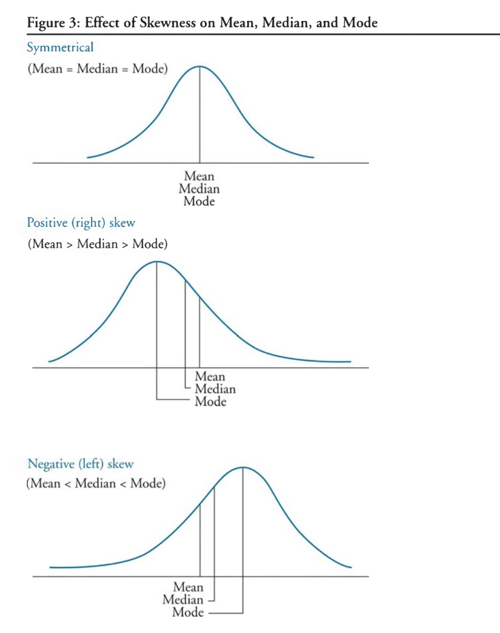
• skewness

  • positively/right skewed distributions: mode < median < mean (for unimodal distribution), positively means more outliner in the positive region

  • negatively/left skewed distributions: mode > median > mode (for unimodal distribution)

    

• kurtosis

  • leptokurtic (more peaked than a normal distribution)
    • great probability of an observed value being either close to the mean or far from the mean
  • platykurtic (more flatter)
  • mesokurtic (same kurtosis)
  • excess kurtosis: kurtosis - 3 (relative to a normal distribution)

Coskewness and Cokurtosis

• coskewness: third cross central moment
• cokurtosis: fourth cross central moment

The Best Linear Unbiased Estimator

LO 16.8: Describe and interpret the best linear unbiased estimator.

• unbiased
• efficient
• consistent
• linear

Distributions

Parametric and Nonparametric Distributions

LO 17.1: Distinguish the key properties among the following distributions: uniform distribution, Bernoulli distribution, Binomial distribution, Poisson distribution, normal distribution, lognormal distribution, Chi-squared distribution, Student’s t, and F-distributions, and identify common occurences of each distribution

The Central Limit Theorem

LO 17.2: Describe the central limit theorem and the implications it has when combining independent and identically distributed (i.i.d.) random variables.

LO 17.3: Describe the i.i.d. random variables and the implications of the i.i.d. assumption when combining random variables.

Mixture Distributions

LO 17.4: Describe a mixture distribution and explain the creation and characteristics of mixture distributions.

Bayesian Analysis

Bayes’ Theorem

LO 18.1: Describe Bayes’ theorem and apply this theorem in the calculation of conditional probabilities

Bayesian Approach v.s. Frequentist Approach

LO 18.2: Compare the Bayesian approach to the frequentist approach

Bayes’ Theorem with Multiple States

LO 18.3: Apply Bayes’ theorem to scenarios with more than two possible outcomes and calculate posterior probabilities

Hypothesis Testing and Confidence Intervals

Applied Statistics

Mean and Variance of the Sample Average

LO 19.1: Calculate and interpret the sample mean and sample variance

Population and Sample Mean

Population and Sample Variance

Population and Sample Covariance

Confidence Intervals

LO 19.2: Construct and interpret a confidence interval

Confidence Intervals for a Population Mean: Normal with Unknown Variance

Confidence Intervals for a Population Mean: Nonnormal with Unknown Variance

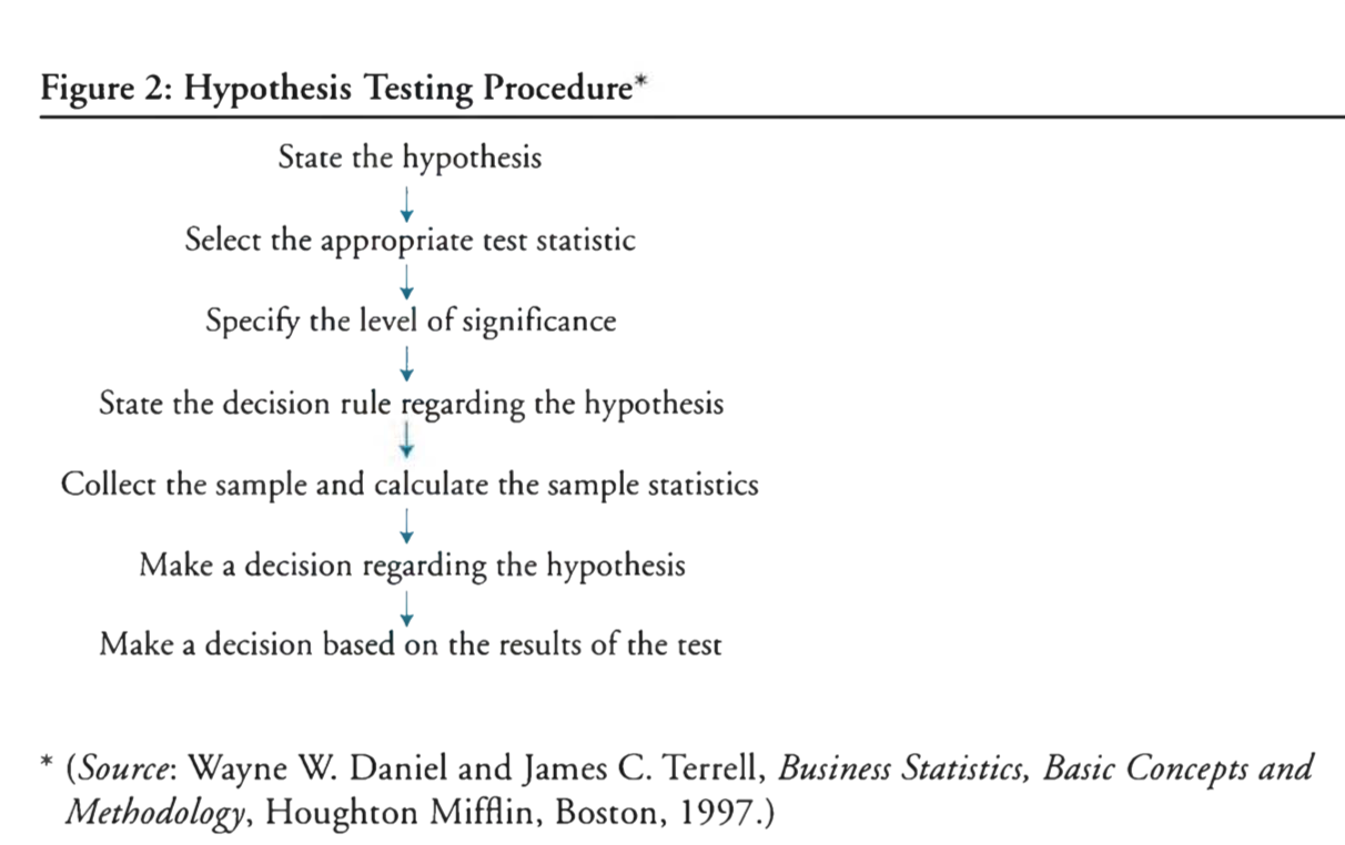
Hypothesis Testing

LO 19.3: Construct an appropriate null and alternative hypothesis, and calculate an appropriate test statistic.

The Null Hypothesis and Alternative Hypothesis

The Choice of the Null and Alternative Hypotheses

One-tailed and Two-tailed Tests of Hypotheses

LO 19.4: Differentiate between a one-tailed and a two-tailed test and identify when to use each test

Type I and Type II Errors

• Type I: rejection of the null hypothesis when it is actually true
• Type II: the failure to reject null hypothesis when it is actually false

The Power of a Test

• power: 1 - P(Type II Errors)

The Relation Between Confidence Intervals and Hypothesis Tests

Statistical Significance v.s. Economic Significance

The p-Value

• p-value: the probability of obtaining a test statistics that would lead to rejection of the null hypothesis

The t-Test

The z-Test

LO 19.5: Interpret the results of hypothesis tests with a specific level of confidence.

The Chi-Squared Test

The F-Test

Chebyshev’s Inequality

• the percentage of the observations that lie within k std of the mean is at least $1- 1/k^{2}$

Backtesting

LO 19.6: Demonstrate the process of backtesting VaR by calculating the number of exceedances.

Linear Regression with One Regressor

Regression Analysis

LO 20.1: Explain how regression analysis in econometrics measures the relationship between dependent and independent variables.

Population Regression Function

LO 20.2: Interpret a population regression function, regression coefficients, parameters, slope, interprect, and the error term.

Sample Regression Function

LO 20.3: Interpret a sample regression, regression coefficients, parameters, slope, interprect, and the error term.

Properties of Regression

LO 20.4: Describe the key properties of a linear regression

Ordinary Least Squares Regression

LO 20.5: Define an ordinary least squares (OLS) regression and calculate the intercept and slope of the regression.

Assumptions Underlying Linear Regression

LO 20.6: Describe the method and three key assumptions of OLS for estimation of parameters.

Properties of OLS Estimators

LO 20.7: Summarize the benefits of using OLS estimators.

• widely used in practice
• easily understood across multiple fields
• unbiased, consistent, and (under special conditions) efficient

LO 20.8: Describe the properties of OLS estimators and their sampling distributions, and explain the properties of consistent estimators in general.

OLS Regression Results

LO 20.9: Interpret the explained sum of squares, the total sum of squares, the residual sum of squares, the standard error of the regression, and the regression $R^{2}$.

• the coefficient of determination (interpreted as a percentage of variation in the dependent variable explained by the indepedent variable)
  • total sum of squares = explained sum of squares + sum of squared residuals (TSS = ESS + SSR)
  • $\sum(Y{i} - \bar{Y})^{2} = \sum(\hat{Y} - \bar{Y})^{2} + \sum(Y{i} - \hat{Y})^{2}$
  • $R^{2} = \frac{ESS}{TSS}$
• difference between “correlation coeficient” and “coefficient of determination” (P137)

LO 20.10: Interpret the results of an OLS regression.

Regression with a Single Regressor: Hypothesis Tests and Confidence Intervals

Regression Coefficient Confidence Intervals

LO 21.1: Calculate, and interpret confidence intervals for regression coefficients.

Regression Coefficient Hypothesis Testing

LO 21.3: Interpret hypothesis tests about regression coefficients

LO 21.2: Interpret the p-value

• p-value: the smallest level of significance for which the null hypothesis can be rejected

Predicted Values

Confidence Intervals for Predicted Values

Dummy Variables

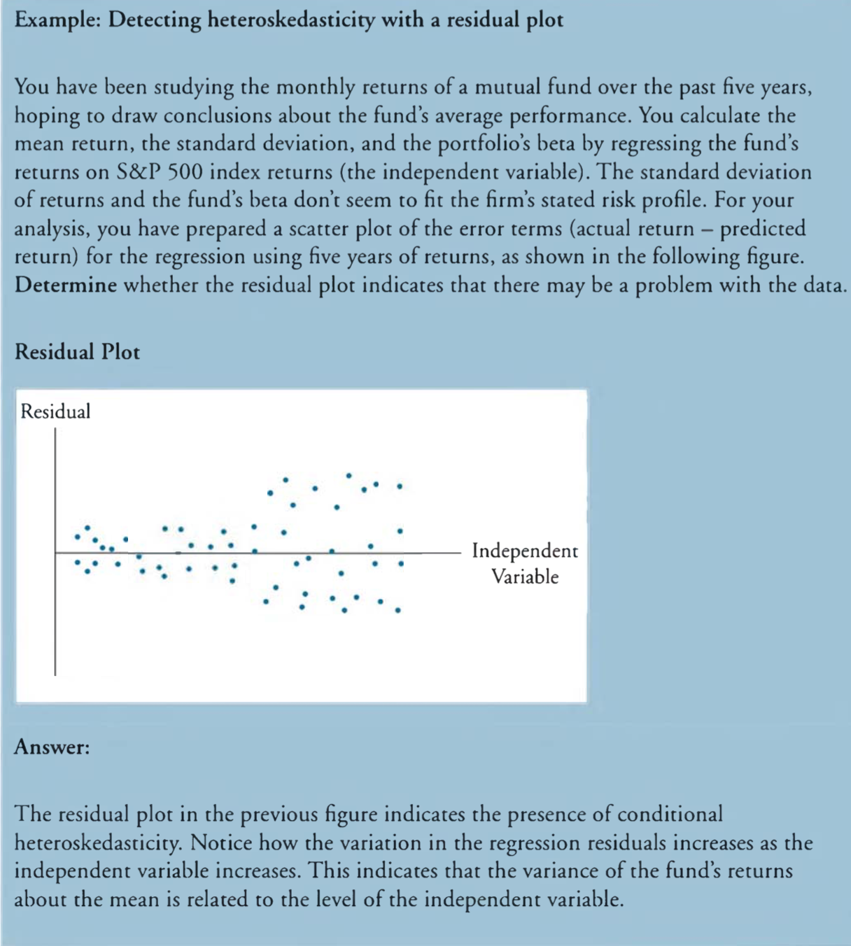
What is Heteroskedasticity?

LO 21.4: Evaluate the implications of homoskedasticity and heteroskedasticity.

• homoskedastic (variance of residuals is constant across all observations in the sample)
• heteroskedasticity (opposite of homoskedastic)
  • unconditional heteroskedasticity (usually causes no major problems with regression)
  • conditional heteroskedasticity (does create significant problems for statistical inference)

Effect of Heteroskedasticity on Regression Analysis

Detecting Heteroskedasticity

Correcting Heteroskedasticity

The Gauss-Markov Theorem

LO 21.5: Determine the conditions under which the OLS is the best linear conditionally unbiased estimator.

LO 21.6: Explain the Gauss-Markov Theorem and its limitations, and alternatives to the OLS.

Small Sample Sizes

LO 21.7: Apply and interpret the t-statistic when the sample size is small

Linear Regression with Multiple Regressors

Omited Variable Bias

LO 22.1: Define and interpret omitted variable bias, and describe the methods for addressing this bias.

Multiple Regression Basics

LO 22.2: Distinguish between single and multiple regression

LO 22.5: Describe the OLS estimator in a multiple regression

LO 22.3: Interpret the slope coefficient in a multiple regression

LO 22.4: Describe homoskedasticity and heteroskedasticity in a multiple regression

Measures of Fit

LO 22.6: Calculate and interpret measures of fit in multiple regression.

Coefficient of Determination, $R^{2}$

Adjusted $R^{2}$

• adjusted $R^{2} = 1 - \frac{n-1}{n-k-1} (1 - R^{2})$ is less than or equal to $R^{2}$

Assumptions of Multiple Regression

LO 22.7: Explain the assumptions of the multiple linear regression model.

Multicollinearity

LO 22.8: Explain the concept of imperfect and perfect multicollinearity and their implications.

Effect of Multicollinearity on Regression Analysis

Detecting Multicollinearity

• high p-value, high $R^{2}$

Correcting Multicollinearity

Hypothesis Tests and Confidence Intervals in Multiple Regression

LO 23.1: Construct, apply, and interpret hypothesis tests and confidence intervals for a single coefficient in a multiple regression.

Hypothesis Testing of Regression Coefficients

Determining Statistical Significance

Interpreting p-Values

Other Tests of the Regression Coefficients

Confidence Intervals for a Regression Coefficient

Predicting the Dependent Variable

Joint Hypothesis Testing

LO 23.2: Construct, apply, and interpret joint hypothesis tests and confidence intervals for multiple coefficients in a multiple regression

LO 23.3: Interpret the F-statistic

LO 23.5: Interpret confidence sets for multiple coefficients

The F-Statistic

• F-statistic: always a one-tailed test, calculated as $\frac{ESS/k}{SSR/(n-k-1)}$

Interpreting Regression Results

Specification Bias

$R^{2}$ and Adjusted $R^{2}$

LO 23.7: Interpret the $R^{2}$ and adjusted $R^{2}$ in a multiple regression

Restricted vs. Unrestricted Least Squares Models

LO 23.4: Interpret tests of a single restriction involving multiple coefficients.

Model Misspecification

LO 23.6: Identify examples of omitted variable bias in multiple regressions.

Modeling and Forecasting Trend

Linear and Nonlinear Trends

LO 24.1: Describe linear and nonlinear trends.

Linear Trend Models

Nonlinear Trend Models

Estimating and Forecasting Trends

LO 24.2: Describe trend models to estimate and forecast trends.

Selecting the Correct Trend Model

Model Selection Criteria

LO 24.3: Compare and evaluate model selection criteria, including mean squard error (MSE), $s^{2}$, the Akaike information criterion (AIC), and the Schwarz information criterion (SIC).

Mean Squared Error

The $s^{2}$ measure

• $s^{2}$ measure (unbiased estimate of the MSE): $s^{2} = \frac{\sum{t=1}^{T} e{t}^{2}}{T-k} = \frac{T}{T-k}\frac{\sum{t=1}^{T} e{t}^{2}}{T}$
• adjusted $R^{2}$ using the $s^{2}$ estimate

Akaike and Schwarz Criterion

• Akaike information criterion: $e^{\frac{2k}{T}} \frac{\sum{t=1}^{T} e{t}^{2}}{T}$
• Schwarz information criterion: $T^{\frac{k}{T}} \frac{\sum{t=1}^{T}e{t}^{2}}{T}$

Evaluating Consistency

LO 24.4: Explain the necessary conditions for a model selection criterion to demonstrate consistency

• the most consistent selection criteria with the greatest penalty factor for degrees of freedom is the SIC.

Modeling and Forecasting Seasonality

Sources of Seasonality

LO 25.1: Describe the sources of seasonality and how to deal with it in time series analysis.

• sources of seasonality
• approaches
  • using a seasonally adjusted time series
  • regression analysis with seasonal dummy variables

Modeling Seasonality with Regression Analysis

LO 25.2: Explain how to use regression analysis to model seasonality

Interpreting a Dummy Variable Regression

Seasonal Series Forecasting

LO 25.3: Explain how to construct an h-step-ahead point forecast.

Characterizing Cycles

Covariance Stationary

LO 26.1: Define covariance stationary, autocovariance function, autocorrelation function, partial autocorrelation function, and autoregression.

LO 26.2: Describe the requirements for a series to be covariance stationary.

LO 26.3: Explain the implications of working with models that are not covariance stationary.

White Noise

LO 26.4: Define white noise, and describe independent white noise and normal (Gaussian) white noise.

LO 26.5: Explain the characteristics of the dynamic structure of white noise.

Lag Operators

LO 26.6: Explain how a lag operator works.

Wold’s Representation Theorem

LO 26.7: Describe Wold’s theorem.

LO 26.8: Define a general linear process.

LO 26.9: Relate rational distributed lags to Wold’s theorem.

Estimating the Mean and Autocorrelation Functions

Lo 26.10: Calculate the sample mean and sample autocorrelation, and describe the Box-Pierce Q-statistic and the Ljung-Box Q-statistic.

LO 26.11: Describe sample partial autocorrelation.

• sample autocorrelation: estimate the degree to which white noise characterizes a series of data
• sample partial autocorrelation: determine whether a time series exhibits white noise
• q-statistics: measure the degree to which autocorrelations vary from zero and whether white noise is present in a dataset
• Box-Pierce q-statistic: reflects the absolute magnitudes of the correlations
• Ljung-Box q-statistic: similar to the above measure

Modeling Cycles: MA, AR and ARMA Models

First-order Moving Average Process

LO 27.1: Describe the properties of the first-order moving average (MA(1)) process, and distinguish between autoregressive representation and moving average representation.

MA(q) Process

LO 27.2: Describe the properties of a general finite-order process of order q (MA(q)) process.

First-order Autoregressive Process

LO 27.3: Describe the properties of the first-order autoregressive (AR(1)) process, and define and explain the Yule-Walker equation.

AR(p) Process

LO 27.4: Describe the properties of a general $p^{th}$ order autoregressive (AR(p)) process.

Autoregressive Moving Average Process

LO 27.5: Define and describe the properties of the auto regressive moving average (ARMA) process.

Applications of AR and ARMA Processes

LO 27.6: Describe the application of AR and ARMA processes.

Volatility

Volatility, Variance, and Implied Volatility

LO 28.1: Define and distinguish between volatility, variance rate, and implied volatility.

The Power Law

LO 28.2: Describe the power law.

Estimating Volatility

LO 28.3: Explain how various weighting schemes can be used in estimating volatility.

The Exponentially Weighted Moving Average Model

LO 28.4: Apply the exponentially weighted moving average (EWMA) model to estimate volatility.

LO 28.8: Explain the weights in the EWMA and GARCH(1, 1) models.

The GARCH(1, 1) Model

LO 28.5: Describe the generalized autoregressive conditional heteroskedasticity (GARCH(p, q)) model for estimating volatility and its properties.

LO 28.6: Calculate volatility using the GARCH(1, 1) model.

Mean Reversion

LO 28.7: Explain mean reversion and how it is captured in the GARCH(1, 1) model.

Estimation and Performance of GARCH Models

LO 28.9: Explain how GARCH models perform in volatility forecasting.

LO: 28.10: Describe the volatility term structure and the impact of volatility changes.

Correlations and Copulas

Correlation and Covariance

LO 29.1: Define correlation and covariance and differentiate between correlation and dependence.

Covariance using EWMA and GARCH Models

LO 29.2: Calculate covariance using the EWMA and GARCH(1, 1) models

EWMA Model

GARCH(1, 1) Model

Evaluating Consistency for Covariances

LO 29.3: Apply the consistency condition to covariance.

Generating Samples

LO 29.4: Describe the procedure of generating samples from a bivariate normal distribution.

Factor Models

LO 29.5: Describe properties of correlations between normally distributed variables when using a one-factor model.

Copulas

LO 29.6: Define copula and describe the key properties of copulas and copula correlation

• copula: creates a joint probability distribution between two or more variables while maintaining their individual marginal distributions.
• copula correlation

Types of Copulas

LO 29.8: Describe the Gaussian copula, Student’s t-copula, multivariate copula, and one factor copula.

Tail Dependence

LO 29.7: Explain tail dependence.

Simulation Methods

Monte Carlo Simulation

LO 30.1: Describe the basic steps to conduct a Monte Carlo Simulation

Reducing Monte Carlo Sampling Error

LO 30.2: Describe ways to reduce Monte Carlo sampling error.

• increase replications
• antithetic variates
• control variates

Antithetic Variates

LO 30.3: Explain how to use antithetic variate technique to reduce Monte Carlo sampling error

Control Variates

LO 30.4: Explain how to use control variates to reduce Monte Carlo sampling error and when it is effective

Resulting Sets of Random Numbers

LO 30.5: Describe the benefits of reusing sets of random number draws across Monte Carlo experiments and how to reuse them.

• Dickey-Fuller (DF) test: used to determine whether a time series is covariance stationary
• Different Experiments:

Bootstraping Method

LO 30.6: Describe the bootstrapping method and its advantage over Monte Carlo simulation.

LO 30.8: Describe situations where the bootstrapping method is ineffective

Random Number Generation

LO 30.7: Describe the pseudo-random number generation method and how a good simulation design alleviates the effects the choice of the seed has on the properties of the generated series.

Disadvantages of Simulation Approaches

LO 30.9: Describe disadvantages of the simulation approach to financial problem solving.